In celebration of pi-day, let’s look at a method of computing pi using random numbers that is often presented in probability, statistics or other classes, as an elementary example of using random sampling and / or simulation.

In my case, the first time I remember seeing / hearing about this example was in a probability class, however we didn’t actually write any code to try it, we just looked at the idea. Later, I was re-introduced to the example when I began to do undergrad ChE research - I was going to be working on a Monte Carlo molecular simulation code for small molecules. When I started, I had no idea what that meant - and one of the first exercises that my adviser gave me, to introduce the idea of computing some physical quantity using simulation, was by chance, this “estimate pi by throwing darts” example.

Estimating Pi by throwing darts

First, this is definitely not an efficient way to approximate pi, but it’s a fun exercise. :)

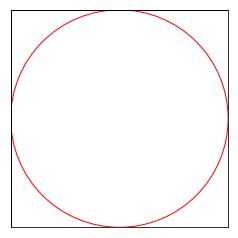
Let’s assume we have a weird dart board, it’s a circle inscribed in a square, where the height of the square is equal to the diameter of the circle, so it looks like this:

We know what the area of the square is $A_s = H^2$ (where $H$ is the height and width of the square). As the circle is inscribed in the square, the diameter, $D$, is $D = H = 2 * radius$.

The area of the circle is of course $ A_c = \pi r^2 $.

We can assume that if we randomly throw darts at this “dart board” that the probability the dart hits within the circle is related to the ratio of the area of the circle to the square. So that,

$$ \frac{P(C)}{P(S)} = \frac{A_c}{A_s} = \frac{\pi r^2}{(H^2)} = \frac{\pi r^2}{4r^2} $$

If we rearrange for $\pi$, we can see that:

$$ \pi = 4 * \frac{P(C)}{P(S)} $$

We can use this result as the basis of our simulation.

Before we start writing any actual code, let’s assume:

• We are so good that we never miss the board completely (or if we do, we don’t count that throw)
• Yet we are still bad enough, that hitting any where on the board is equally likely. That is to say, despite any attempt aiming at a specific point, we’re no more likely to hit that point than any other spot on the board.

The idea is that we will randomly throw darts, and keep track of how many land within the circle (and the square), and how many land only within the square, but not the circle. Assuming that we never miss the board, every dart is within the square.

So with our simulation, we just have to throw a ton of darts, keep track of the results, and use that to calculate the fraction of times the dart lands within the circle (and multiply by 4 as above) to estimate pi.

An example

You can find a full example of one way to do this in Python3 on GitHub, here is what the main loop looks like. It references helper functions that are defined at the start of the file, but this should give a pretty good idea of how it works:

while throw_counter < number_of_darts_to_throw:
        
    # Make a random dart and throw it...
    x, y = throw_dart(R)
    throw_counter += 1
        
    # ...it hits the board, is it within the circle?
    in_circle = is_within_circle(x, y, R)
    hit_counter += in_circle
        
    # Now we add the point to the plot...
    add_to_plot(x, y, R, in_circle)

# Calculate pi estimate    
pi = 4.0 * (hit_counter / throw_counter)

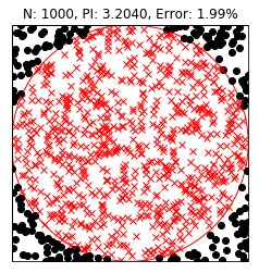
So we can run this for different numbers of darts, and as you probably guessed, “throwing” more darts tends to give a closer approximation to pi. Here are the results with 1000 darts - red x’s are darts that are hits (within the circle), while black circles are misses (outside the circle):

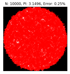
verses with 10000 darts:

Clearly we’re getting a much closer approximation in the second case.

Conclusion

This is a cool example that, though is definitely not efficient for approximating pi, provides a starting point for using “random” numbers to perform a simulation and then use the results of that simulation to compute something “physical”. Also if you aren’t familiar with the Python3 plotting module, matplotlib, this example will also demonstrate how to plot some shapes, and how to plot scattered x, y points with different colors and markers.

As I mentioned above, this example was given to me as a starting point for understanding Monte Carlo integration, and then eventually Monte Carlo simulation. Maybe some future posts will demonstrate some examples of those types of simulations.