TL;DR - “real” gases heat up or cool down when they are throttled through a valve from high pressure to low pressure. This is because of interactions between the molecules and it’s an interesting property. Counter intuitively, maybe, they flip from cooling to heating at some temperature. A one plot summary in two plots: interactive plot
Motivation
I read a blog post from a researcher hypothesizing about the mechanism behind the Joule-Thomson effect. I don’t agree completely with his hypotheses in the post (that repulsive forces don’t matter), but it got me thinking about it a lot. Haven’t looked at this stuff in a while, and ever so often I’m reminded how cool (🥁) it is. Thought it might be worth sharing some of some of the thoughts and figures I made after knocking the dust off my old stat mech book and playing with some simple models.
Who is this for?
I’m trying to write this for a broad audience - using conversational language. I am going to show some of the equations, but not going to go too deep into the details. Most of the thermodynamics is something you would see in an undergraduate engineering thermodynamics course. With the exception maybe of the connection of the second virial coefficient to the pair potential, which is something you are more likely see in a statistical mechanics or statistical physics course, or maybe physical chemistry.
My goal with writing about this it to try to explain it in a really accessible way - and if you want to dig more deeply - I’ve included some references, and code I used to make the figures, etc.
Fair warning - I might be slightly imprecise in the explanation here and there, most of the time it’s because I couldn’t find a good way to keep it clear without a bunch of jargon. The rest of the time, I probably just got it wrong. I’m always happy to hear your thoughts and feedback though!
Joule-Thomson Effect
When real gases are throttled through a valve from high pressure to low pressure, they change temperature. Most gases at ambient conditions cool, but some actually heat up instead. That’s the whole thing really.
Here’s the wiki for the Joule-Thomson effect.
Why it’s interesting?
Some questions:
- why does it change temperature at all? –> because of interactions between the molecules
- why does it flip from cooling to heating? –> because of the interplay between attractive and repulsive forces
- Is it useful? –> yes, it’s used to liquify gases in some applications
To me the interesting part is that whether the gas cools or heats when it is throttled depends on the temperature of the gas. We can adjust this starting temperature, changing nothing else about the process, and we’ll get heating instead of cooling. The temperature at which this happens is called the inversion temperature.
How it works
There’s actually two things going on in the Joule-Thomson expansion - so to understand it better, let’s look at Joule expansion first.
Joule expansion
Joule expansion is a free expansion of a gas into a vacuum. There is no work done on or by the gas (this is the main difference from the Joule-Thomson expansion).
Still, like the Joule-Thomson expansion, real gases change temperature in this process - and can also have an inversion temperature where the temperature changes sign. For example, the usual suspects like Helium and Hydrogen heat up under Joule expansion at ambient temperature, but cool at lower temperatures.
When the gas molecules are interacting with each other, they act like little magnets at some ranges - attracting each other. But if they get too close, they strongly repel each other. The “potential energy” of the system here then just depends on how close each molecule is to each other molecule on average. Of course on the the high pressure side, they are closer and the potential will be more affected by interactions between the molecules than on the low pressure side where they are further apart.
If the interactions are mostly repulsive, the molecules are all repelling each other so the potential energy is higher on the high pressure side than on the expanded side. That potential energy is converted to kinetic energy when the gas expands and so the temperature increases.
On the other hand, if it’s mostly dominated by attractive forces, the potential energy is lower on the higher pressure side. There is a cost to be paid to spread them out. That cost is paid out of the kinetic energy of the gas, and the temperature decreases.
Real gases are a mix of both attractive and repulsive forces. Strongly repelling each other when very close, and then attracting each other for much longer distances. Give that we have both repulsive and attractive forces, the Joule and Joule-Thomson expansions can show either cooling or heating, depending on the starting temperature of the gas.
Joule-Thomson expansion
In the Joule-Thomson expansion, we have two key things happening:
- (1) flow work ($\Delta (PV)$) - any little chunk of gas on the high pressure side is doing work to push the little chunk of gas in front of it through the valve. Any little chunk of gas on the low pressure side is doing work to push the little chunk of gas in front of it out of the way and down the line. This is what makes it different from a free expansion (where no work is done)
- (2) change in potential energy $\Delta U_{pot}$, due to the change in the average distance between the molecules (just like in the Joule expansion)
The constraint changes too - Joule-Thomson expansion happens at constant enthalpy H = U + PV, not constant U (as in the Joule expansion), and the sign of $μ_{JT}$ comes out of competition between these two pieces (not just the change in potential energy).
For fun - and with some reasonable assumptions and simplifications, we can look at some simple cases of different types of interactions between the gas molecules and see how they qualitatively affect the Joule-Thomson coefficient and the inversion temperature (the place it changes from cooling to heating / flips sign) - if it ever does.
How can we model it?
To bridge the gap between the micro (molecules) and macro (Joule-Thomson coefficient) scales, we can borrow some tools from statistical mechanics. We are also going to need to assume the our interactions between molecules are dominated by interactions between pairs of molecules, and not interactions between clusters of 3 and more molecules. This is a reasonable assumption until pressure becomes very high. It’s certainly good enough to give us some of the qualitative, directional results we’re after here.
Pair potentials
There are a bunch of different potential functions that people often use for modeling these interactions, all with different specific uses.
We can look at a cases with:
- no interaction (ideal gas)
- only “repulsive” interaction (hard sphere) - they just can’t overlap
- only “repulsive” interaction (soft sphere) - they can’t get too close
- only attractive interaction (square well) - they want to close, but after a certain point it doesn’t matter anymore
- both attractive and repulsive interaction (Lennard-Jones) - most realistic - they repel each other (soft sphere) at short distances, and attract each other at longer distances
Here’s an example of what they look like, where the ‘r’ on the x-axis is the distance between the centers of the two molecules, and the ‘U’ on the y-axis is the potential energy of the interaction between the two molecules according to the chosen potential function.
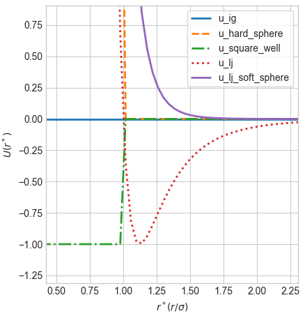
Ideal gas they don’t interact, so the potential energy is zero. The hard sphere they don’t interact, unless they get too close and the potential energy is infinite. The soft sphere is the same, but it ramps up more slowly. The square well is attractive, but it’s only attractive if the distance is less than a certain threshold, after which it’s zero. The Lennard-Jones is a mix of attractive and repulsive, overall it’s attractive if the distance is greater than a certain threshold, and repulsive if it’s greater than that threshold - and a mix in between. So there’s a sweet spot where we have a minimum in the potential energy (check out the plot above).
Virial expansion
I’m not going to work through the derivation here, but you can actually arrive at the Virial expansion from a first principles approach using statistical mechanics (See McQuarrie’s Statistical Mechanics - Chapter 12-1).
$$ P = \frac{RT}{V} \left(1 + \frac{B(T)}{V} + \frac{C(T)}{V^2} + \cdots \right) $$
Where $P$ is the pressure, $R$ is the ideal gas constant, $T$ is the temperature, $V$ is the volume, and $B(T)$, $C(T)$, etc. are the virial coefficients, which are functions of temperature.
This gives us a relation for pressure of a gas as a function of the temperature and volume (called an Equation of State - EOS). Infinite terms is a lot so we’re going to quickly make it less rigorous and easier to work with by truncating it after the second term, like:
$$ P = \frac{RT}{V} \left(1 + \frac{B(T)}{V} \right) $$
This is a good enough approximation for our purposes, until pressure is very high.
See for example, this table from McQuarrie’s Statistical Mechanics that shows the second and third virial coefficients (plus the sum of remaining terms) for Argon at 1-1000 atm:
| $p$ (atm) | $\frac{p}{\rho kT}$ (Z) |
|---|---|
| 1 | $1 - 0.00064 + 0.00000 + \cdots (+0.00000)$ |
| 10 | $1 - 0.00648 + 0.00020 + \cdots (-0.00007)$ |
| 100 | $1 - 0.06754 + 0.02127 + \cdots (-0.00036)$ |
| 1000 | $1 - 0.38404 + 0.68788 + \cdots (+0.37232)$ |
Source: E. A. Mason and T. H. Spurling, The Virial Equation of State (New York: Pergamon, 1969). Reproduced without permission. YOLO.
Connecting B(T) to U(r)
Statistical mechanics (the derivation can be found, you guessed it, in McQuarrie’s Statistical Mechanics - Chapter 12-1) gives us a way to relate the second virial coefficient to the pairwise interactions energy between pairs of molecules.
It’s given by:
$$ B(T) = -2\pi\int_0^\infty \left(e^{-\frac{U(r)}{k_BT}} - 1\right) r^2 dr $$
Where $U(r)$ is the potential energy of the interaction between the pairs of molecules, and $r$ is the distance between the centers of the two molecules.
The third and higher virial coefficients that we hand waved away are related to three body, four body, etc, interactions between molecules. Fortunately, there are lot of conditions where we can ignore them - at least for now to look at the qualitative physics. See the table above for Argon for when this works and when it start to get shaky (high pressures - three body interactions start to matter).
For any given pair potential, at a given temperature, we can calculate the second virial coefficient by evaluating the integral above. Some of them have analytic solutions, they can also be evaluated numerically using your favorite numerical integration method (or just scipy.integrate.quad if you’re lazy).
Finally - compute $\mu_{JT}$
The expansion we’re doing is at constant enthalpy, and also by definition the Joule-Thomson coefficient describes how the temperature changes with pressure at constant enthalpy and is given by:
$$ \mu_{JT} = \left( \frac{\partial T}{\partial P} \right)_{H} $$
Where $H$ is the enthalpy. There is another derivation I’m sparing you here, but it’s even given on the wiki page for the Joule-Thomson effect (link).
Basically, as it’s given it’s not written in a friendly way - it would be better if we can could rewrite it in terms of things we can easily measure or model like the pressure, temperature, and volume. Doing that we end up with an expression in terms of derivatives that are easier to compute. Especially, if we have a model for say, how pressure relates to temperature and volume - like the virial expansion we just sorted out above!
Following that linked derivation gives us:
$$ \mu_{JT}C_p = T\left( \frac{\partial V}{\partial T} \right)_{P} - V $$
Now we want to make one more substitution to make things simpler to actually compute. We’ll apply the triple product rule to change the volume derivative to a pressure derivative - because of the way the virial expansion is written - it looks more complicated but the derivatives are easier to compute.
So $\mu_{JT}$ we end up with:
$$ \mu_{JT}C_p = T\frac{\left(\frac{\partial P}{\partial T} \right)_{V}}{\left(\frac{\partial P}{\partial V}\right)_{T}} - V $$
Which, after differentiating the virial expansion, plugging in, and rearranging, gives us:
$$ \mu_{JT}C_p = \frac{TB^\prime(T) - B(T)}{1 + 2\frac{B(T)}{V}} \approx TB^\prime(T) - B(T) $$
Where $B’(T)$ is the derivative of the second virial coefficient with respect to temperature. We’ve dropped the denominator term because it won’t change the sign of $\mu_{JT}$ and we only really care of the physics not the magnitude. It’s near 1 for most conditions, B(T) is small relative to V.
Now we finally have an expression for $\mu_{JT}$ that directly depends on the temperature and underlying pair potential.
Results
Now we can compute $\mu_{JT}$ for different pair potentials by evaluating the integral for $B(T)$ for each potential. Let’s do it for the potentials we looked at above:
- no interaction (ideal gas)
- only repulsive interaction (hard sphere)
- only repulsive interaction (soft sphere)
- only attractive interaction (square well)
- both attractive and repulsive interaction (Lennard-Jones)
Here’s what the resulting $\mu_{JT}$ looks like for each potential, as a function of temperature:
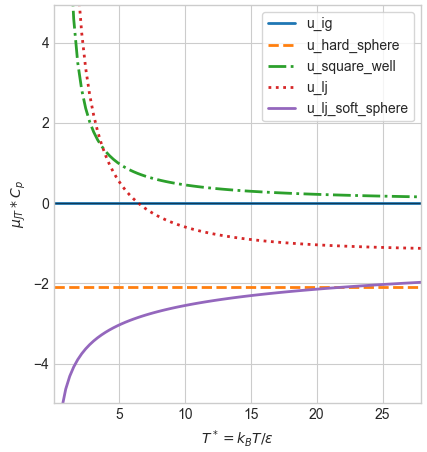
Pretty cool right? We have:
- (1) the ideal gas - it’s always zero. The molecules don’t interact and we don’t have change in potential energy when they expand
- (2) the hard sphere potential - there are only repulsive interactions - the gas always heats up when it expands
- (3) the soft sphere potential - there are only repulsive interactions - the gas always heats up when it expands
- (4) the square well potential - there are only attractive interactions - the gas always cools when it expands
- (5) the Lennard-Jones potential - it’s a mix of attractive and repulsive interactions - it’s positive at low temperatures, negative at high temperatures, and zero at an intermediate temperature. So that at first when attractive forces dominate at low temperature, it cools, but then, after the inversion temperature, when repulsive forces dominate, it heats up instead
Notes
Both purely repulsive potentials heat on expansion. I included the hard sphere alongside the soft sphere because they isolate different pieces of the mechanism. The hard-sphere potential is either zero or infinite, there’s no in-between. So in Joule (free) expansion the hard sphere does nothing for the potential energy. Even we have a repulsion potential and the molecules can’t overlap, the average potential energy is zero at any temperature, so there’s no potential energy to convert into kinetic energy. But in Joule-Thomson, the hard sphere still heats up. And since $\Delta U_{pot} = 0$, that heating must come entirely from the $-\Delta (PV)$ (flow work) term. I believe the hard sphere is the cleanest possible demonstration that flow work alone can drive JT heating. The molecular interactions affect the PV via B(T), a constant in this case. Essentially some of the volume is “excluded” by the “hard sphere” shape of the molecules. The soft sphere is the next because it’s very similar - but the wall is finite, so configurations where molecules sit partway up the wall do actually contribute to the potential energy. How often those configurations show up depends on temperature. So now there is a real $\Delta U_{pot}$ in free expansion. The gas heats from that alone, and in JT the $-\Delta (PV)$ piece piles on top, heating it even more.
I made a simple adjustable plot in JS (vibe coded by pointing cursor at my python code) - if you adjust the ratio of attractive to repulsive interactions, for example for the LJ potential, you can see how the inversion temperature changes.
You can play around with it here: link to the plot
I tested it out for some real gases using united atom Lennard-Jones parameters for them I found online in various places - not really a quantitative match, but the trend between gases is correct.
For example, Helium’s inversion temperature is super low (below room temperature for any room anywhere basically), and Hydrogen’s is pretty low (below room temperature for most rooms)
- while N2 and CO2 are higher (above room temperature unless your room is an oven / furnace).
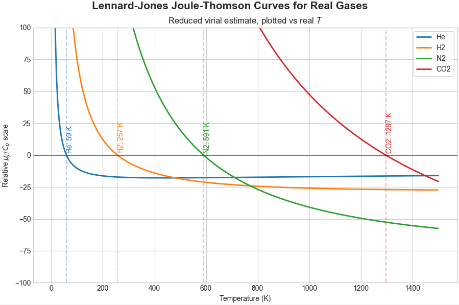
I’ve seen that Helium and Hydrogen in particular, at low temperatures, would need quantum effects to be taken in account, so the purely classical model approach doesn’t cut it for a quantitative match.
I’m sure you can get more quantitative results using empirical or semi-empirical Equation of State models - but that’s less interesting in my opinion. They’re just regressed to data - usually saturated liquid density and saturation pressure data - and more for the more sophisticated models.
Conclusion
That’s it for now! If you found this interesting, and you’re not a robot, I would love to hear your thoughts.
References:
- McQuarrie’s Statistical Mechanics
- Albarran-Zavala et al. Joule inversion temperatures for Some simple real gases. link
- Python script for figures