TL;DR - Using a Markov Chain to model your historical sales pipeline data can help you understand the probability of eventually closing a deal based on (1) the stage the opportunity is currently in and (2) your historical data. This lets you estimate the future value of your current pipeline based on your own past data.
What is a Markov Chain?
It is a mathematical model used to describe how probabilistic systems or processes evolve over time. They have been used to model all kinds of processes in fields ranging from physics and chemistry, to economics and finance. They can even be used to model games of chance (Snakes and Ladders, etc). Here, we look at a sales pipeline as a discrete Markov Chain.
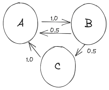
The main idea is that you have a number of “states” - each representing a specific situation. In the figure below, there are three states, A, B, and C. Everytime we advance a “timestep”, there is a certain probability to transition from one state to another state. For example, if you start in state A in the figure below, there is a 100% probability of moving to state B. However, starting in state B, there is a 50% probability of going to state A or C.

The most interesting feature of this model, and what makes it a “Markov” chain is that it depends only on the current state of the system - it has no “memory” and from any current state you can move the model forward without needing any knowledge of the previous state(s) of the system.
The states of the system can represent almost anything, but for the sake of this blog, our “states” represent where the prospect or lead is in the sales process. So for example, something like: “Identified”, “In discussion”, “Quoted”, “Forecasted”, “Closed Won”, and “Closed Lost”. As we advance, there is some probability or chance that a lead in any “state” will move to any other state - so say a “Forecasted” lead has a 70% probability to end up in “Closed Won” and 30% in “Closed Lost”.
Applying the Model to Sales Data
So how can you use this model? Imagine you have something like the stages listed above in your CRM (Salesforce, Hubspot, etc) applied to your opportunities. Let’s imagine the breakdown of open opportunities is something like:
| Opportunity Stage | Number of Opportunities |
|---|---|
| Identified | 200 |
| In discussion | 100 |
| Quoted | 50 |
| Forecasted Win | 20 |
It would be useful to know, based on your own historic data, what the chances of an opportunity eventually closing won are, based on the stage it is in. With this information - the future value of the current pipeline based on historic close probability can be calculated. The tricky part - stages can be skipped, and they don’t go straight to “Closed Won” normally, especially in the earlier stages. For example - it’s easy to calculate the ratio of opportunities that moved from “Identified” to any other stage directly, but computing their overall chances of being “Closed Won” can be a little tricky. It can be done without the Markov Chain approach by solving iteratively - but the Markov Approach is more intuitive and eventually allows you to add time based simulation based on your data.
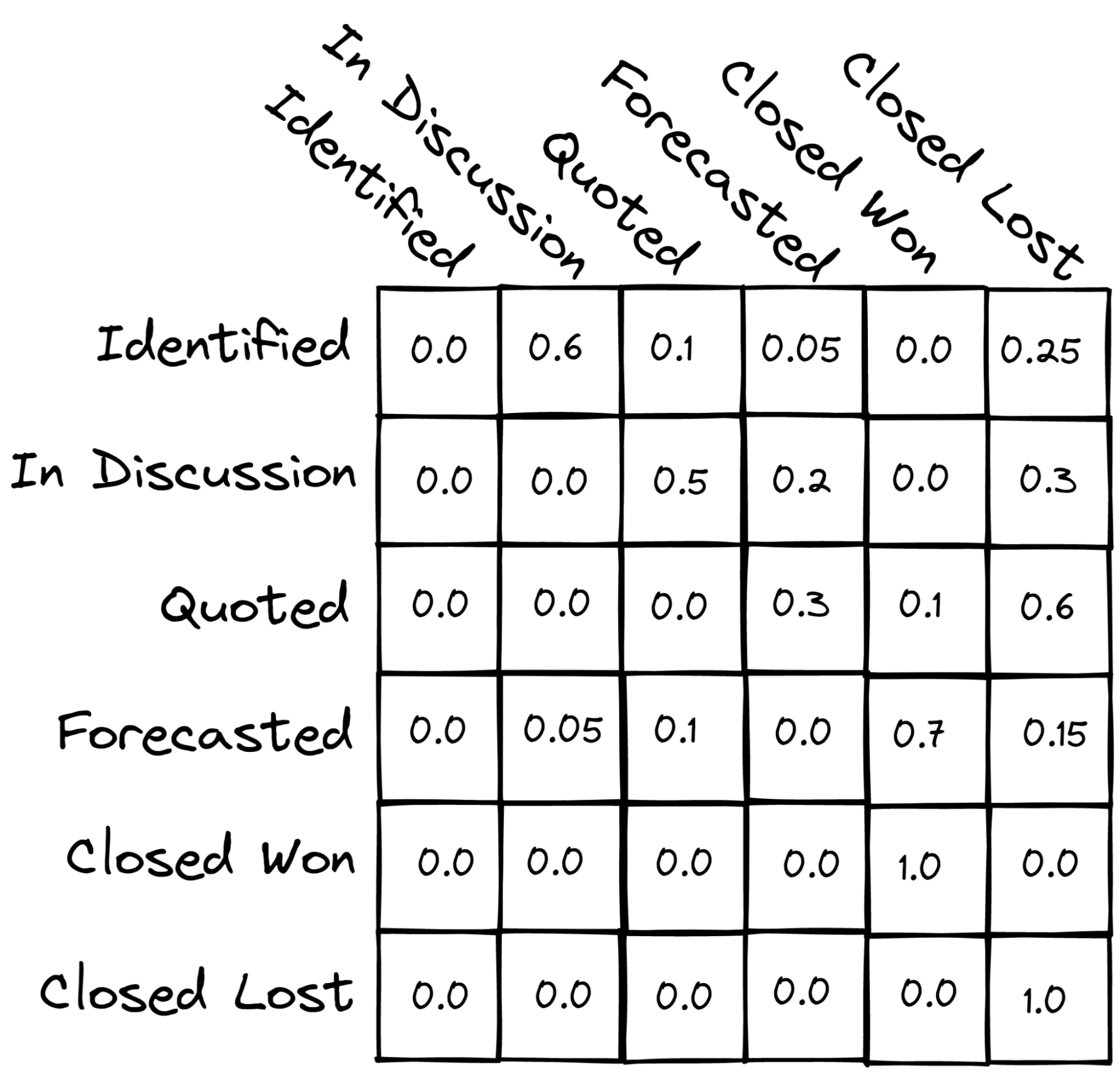
First you need the overall probability of going from any one to any other stage, including going backwards if that is possible. This is the “transition probability” in the sense of the Markov Chain, and it turns out to be useful to put the transition probabilities into a matrix (the “transition matrix”). It might end up looking something like this (numbers entirely fabricated):
I made this image using excalidraw

You can see that the columns and rows each represent a stage - each element represents the probability of moving from the stage represented by that element’s row to the stage represented by that element’s column. So for example, in the image above, there is a 0.6 probability (60% chance) that an opportunity in “Identified” goes to “In discussion”, 0.1 probability of going to “Quoted”, etc. In our example, we included “Closed Won” and “Closed Lost” stages as “sinks” - once an opportunity moves to one of these states, it will never move out (e.g. it’s closed). Using a transition matrix like this, we can start with a current distribution of open opportunities in different stages as shown in the table above and we will eventually end up with all of the opportunities in either “Closed Won” or “Closed Lost” - which is what we expect!
To advance to the next step with a Markov Process, the current distribution is multiplied by the transition matrix. Doing that over and over continually moves opportunities through the pipeline according to the estimated probabilities until they end up in either “Closed Won” or “Closed Lost”. In a simple way, that gives an estimate of the value of the current opportunity pipeline - e.g. an idea of how many of the open opportunities, despite their current stage, will end up “Won” versus “Lost”. Note: this is only the case for our application as we have two states that will gobble up the opportunities (Closed Lost and Closed Won). However, it’s also possible that there is a stationary or equilibrium distribution for a given transition matrix, that the system will converge to.
Part 1 of this Gist shows how to do this in Python using the example data given here (the distribution in the table and transition matrix in the above figure).
However, it doesn’t yet tell us two important pieces of information - the overall probability of an opportunity to end in “Closed Won” from any stage, and we have no concept of “how long” it will take for these opportunities to evolve.
Estimating Each Stage’s Overall Chance of being Won
Let’s assume that the transition matrix above was computed using historical data from some CRM (Salesforce, Hubspot, etc). It would be great to use our actual data to compute the probability that an opportunity ends up being won based on its current stage, and we can do that using the Transition Matrix we have created! Just set the initial distribution of opportunities to only consist of the stage you are interested in computing the probability of, and take Markov Steps until all the opportunities have moved to either Close Won or Closed Lost. You can then do this for each stage to get their overall close probability. You can do this in Python as shown in part 2 of this Gist.
For the example data we used we get that each stage has the following close probability:
| Opportunity Stage | Overall Probability of “Closed Won” |
|---|---|
| Identified | 0.26 |
| In discussion | 0.31 |
| Quoted | 0.32 |
| Forecasted Win | 0.75 |
So this means that, in our historical data (remember we used that for the transition matrix) an opportunity that was “In discussion” ended up being won 31% of the time. This value can be plugged into the CRM you are using (at least it’s no problem in Salesforce) to help you estimate the expected future value of your pipeline. This could be useful for production planning and other forecasting activities, but we still don’t have any concept of “when” these deals might close.
Estimating Time to Close and Other Improvements
The overall close probability for each stage is useful to estimate, but it would clearly be even better to have an idea of how your opportunity pipeline may change as a function of time. To add this aspect into the simulation, we need to pull out another piece of data related to the average time that an opportunity spends in a given stage. I am still working out the kinks with the best way to represent this in a way that is consistent with our original computed probabilities, so that the time based simulation and the overall solution end up with the same result - but that’s material for another day!
Give enough data, especially if you’re working with a large volume pipeline - the prospects could be grouped into more detailed segments. For example, maybe you serve multiple sectors and they have very different close ratios, etc. It would also be interesting to incorporate data from customer interaction details (emails, calls, etc), though I’m not sure in my case that I have enough data.