Modeling Sales Pipeline using Monte Carlo Simulation

TL;DR - Monte Carlo Simulation can be used to model your historical sales pipeline data to account for some of the randomness and uncertainty in the sales process. In this post, Monte Carlo Simulation is introduced and then applied to the same case introduced in a previous post.

What is Monte Carlo Simulation?

Monte Carlo Simulation is used to simulate a process using random sampling. It is a very general technique that can be used to model all kinds of processes in fields ranging from physics and chemistry, to economics and finance. In previous posts, I used Monte Carlo Simulation to Play ‘Shut the Box’ and to estimate the value of pi. Here, I use it to approach the sales pipeline model introduced in a previous post differently. Basically, that approach used a Markov Chain to model the sales pipeline. The probabilities used in the Markov Chain were computed from the data, and understood to represent the overall average probability of moving from one stage to another, or at least the best we could do to estimate that probability. Even if we were right about those probabilities on average, a lot of different outcomes are possible for a given starting distribution of opportunities. Normally, we would use Monte Carlo simulation to randomly sample from these possible outcomes (eg the posts above about Pi and Shut the Box). The most probable outcomes will show up more in our simulation steps than the less probable ones, and we can compute the average and estimate a confidence interval for the results. In the examples here, we already know the results for the average case. We’ll see that we can also get a sense of the range of possible outcomes and visualize what the variance in the randomly sampled value means for range of output values in some other variable.

Coin Example

As an example, the probability of flipping heads on a fair coin is 0.5, but if you flip a coin 10 times, you might get 7 heads and 3 tails, or 5 heads and 5 tails, or 10 heads and 0 tails, etc. Obviously some of those outcomes are more likely than others, but they are all possible. Monte Carlo is a way to explore all the possibilities using random sampling. As an example, we can flip 10 coins 1000 times and keep track of how many heads we get each time. Here’s some Python code to do that:

import numpy as np

def flip_coin():
  return 1 if np.random.uniform() > 0.5 else 0

num_coins = 10
num_sims = 1000

results = {}
for i in range(num_sims):
  results[i] = np.sum([flip_coin() for _ in range(num_coins)])

vals = list(results.values())
print(f"Max: {np.max(vals)}, Min: {np.min(vals)}, Avg: {np.mean(vals)}")

The output will be different each run because it’s random. You can see that even though we expect that on average we have 5 heads and 5 tails, we can get a lot of different results depending on our random sampling.

In some cases, you’ll see that the maximum number of heads was 10, the minimum was 0, and the average was 5.03 - so on average we always get pretty close to the expected value of 5 heads, but at least once we flipped 10 coins and got no heads, and another time we got 10 heads!

The goal of applying Monte Carlo simulation to a process is often to explore these different possible scenarios and evaluate their relative probabilities. Of course, this can be computed in the coin example, but is often hard or impossible to compute in other cases.

Monte Carlo Simulation of Investment Returns

As another example, let’s say you have a portfolio of investments that you expect to return 8% on average, but you know that the actual returns will vary from year to year. Of course you can use the annuity formula and compute the what you expect the future value to be based on the average (8%) return, but what happens if we run Monte Carlo Simulations to see what’s possible as the rate fluctuates?

Here’s that the normal case looks like (starting with $0, contributing 5k per year, 8% interest, and 30 years):

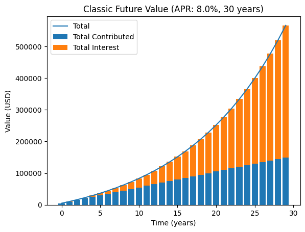
So using these assumptions, we expect to have about $566416.06 in 30 years. But what if we run Monte Carlo Simulations to see what’s possible as the rate fluctuates every year?

Here’s the link to the Python code to do the work. And here’s the main function that runs the simulation:

def run_mc_simulation(
    starting_value=starting_usd,
    yearly_contribution=yearly_additions_usd,
    average_rate=average_interest_rate,
    std_dev_rate=std_dev_rate,
    years=time_in_years):
  stats = {}
  accumulated_interest = 0.0
  current_value = starting_value
  for year in range(years):
    rate = np.random.normal(average_rate, std_dev_rate)
    interest_this_period = current_value * (rate / 100)
    current_value += (yearly_contribution + interest_this_period)
    accumulated_interest += interest_this_period
    stats[year] = dict(
        contributed=(year+1) * yearly_contribution,
        interest=accumulated_interest,
        rate=rate,
        current_value=current_value)
  return stats

You can see the results after we run 100 simulations. On average, we end with an amount pretty similar to what we expected.

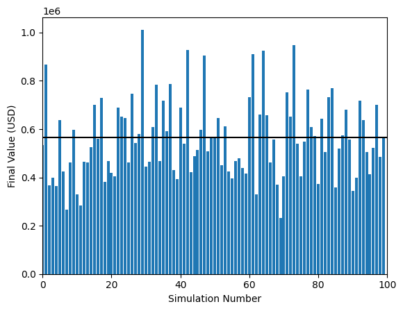
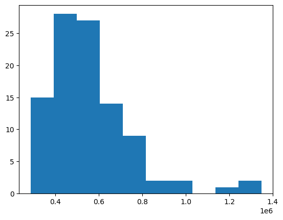
But there is a lot of variation simulation to simulation - sometimes we end up with a lot more (~$1M), sometimes a lot less ($230k)… All based on our luck! Here’s a histogram of the results:

I encourage you play with the standard deviation and rate (try running in this Google Colaboratory Notebook)

Using the simulation approach, we can look at the range of possibilities based on the uncertainty in the rate of return we expect to earn from year to year. In our simple sales pipeline case, we can use Monte Carlo to explore the different possible outcomes of the sales pipeline assuming there is some uncertainty in the sales process, or in our estimated transition probabilities. We already know what the we get using the average transition probabilities - but let’s see what we get using Monte Carlo!

Monte Carlo Simulation of the Sales Pipeline

In the previous post, we used a Markov Chain to model the sales pipeline. The probabilities used in the Markov Chain were computed from the data, and understood to represent probabilities of an opportunity in one stage to move to another stage. We just need to make some updates to the script we used in the previous post to use Monte Carlo Simulation instead of updating the distribution using the transition matrix. Here’s the updated script:

This is the main function that runs the simulation (the full context is in the gist linked above)

def perform_mc_sim(op_dist, transition_matrix):
  """ Run Monte Carlo simulation using estimate probabilities

  - Take each individiual 'opp' in the i'th stage
  - Move it to one of the possible j'th stages based on the transition matrix
      * This time, a random number is generated from a uniform distribution and
        we only move if the random number is less than the transition
        probability. So the average transition probability is the same as our
        transitition matrix, but we can incorporate randomness
  - Keep going until all the 'opps' are in "Closed Won" (index -2) or in
    "Closed Lost" (index -1)

  Returns the overall fraction of opportunities ending in "Closed Won"
  """
  op_types = len(op_dist)
  while np.sum(op_dist[-2:]) < np.sum(op_dist):
    # for each stage, take each op and decide where it moves randomly according
    # to the averages in the transition matrix
    for i in range(op_types):
      # for each actual opportunity in this stage, decide where to move it
      for _ in range(op_dist[i]):
        # generate random number (uniform)
        random = np.random.uniform()
        # check against each possible move in the transition matrix
        transition_prob = 0.0
        for j in range(op_types):
          if op_dist[i] <= 0:
            break
          prev = transition_prob
          # Note: we add here and then check that the random number is betwen
          # this probability and the last one we checked, eg if the they are:
          # [0.5 0.25 0.25 ... 0.0], if the random number is between 0 and 0.5 we
          # got to stage "0", if it's between 0.5 and 0.75 we go to stage "1",
          # etc
          transition_prob += transition_matrix[i][j]
          if prev < random < transition_prob:
            op_dist[i] -= 1
            op_dist[j] += 1
            frames_for_animation.append(op_dist.copy())
            break
        break
  return op_dist[-2]/np.sum(op_dist)

The script keeps going and move opportunities around until all of them end up in either “Closed Lost” or “Closed Won”. It also creates an an animation of the evolution of the distribution of opportunities over time:

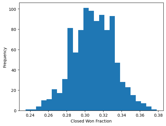
If we run it 1000 times, we get the following stats for the overall probability of an opportunity ending in “Closed Won”, given the starting distribution of opportunities and the approximate transition probabilities:

For comparison, in the Markov Chain post, we used just the average transition probabilities and got the following that 0.31 of the opportunities would end up in “Closed Won”. So we can see that using Monte Carlo Simulation, we get a similar result on average, but there are some runs where we get a much higher or lower probability of ending in “Closed Won” (0.38 or 0.24, respectively).

We can even create a histogram of the results to see the approximate frequency of each value of “Closed Won”:

Using this approach, bounds can be attached the “value” of the pipeline based and other scenarios can be explored in addition to the average case.

Conclusion

To go even further, it would be possible test the sensitivity to the estimates of the transition matrix probabilities by simply perturbing them randomly by up a fixed amount and observing the changes to the results. Further the model could be updated as real world sales data is collected to improve the estimates of the transition matrix probabilities. Maybe we’ll tackle that next…

If you have any questions or comments, please reach out!