TL;DR: A quick “non-mathematical” introduction to the most basic forms of gradient descent and Newton-Raphson methods to solve optimization problems involving functions of more than one variable. We also look at the Lagrange Multiplier method to solve optimization problems subject to constraints (and what the resulting system of nonlinear equations looks like, eg what we could apply Newton-Raphson to, etc).
Introduction
Optimization problems are everywhere in engineering and science. If you can model your problem in a way that can write down some function that should be minimized or maximized (the objective function) to get the solution you want, even in cases where there is no analytical solution (most real cases), you can often obtain a numerical solution.
You can find critical points of a function (minima, maxima, and saddle points) by differentiating the function and setting the derivatives to zero. When you have a function of just one variable, this is pretty straightforward and you end up with a single equation to solve. When you have a function of multiple variables, you end up with a system of equations to solve. For example, if you have a function $F(x, y)$ and you want to find the critical points, you need to solve the system of equations:
$$ \partial F/\partial x = 0 \quad \text{and} \quad \partial F/\partial y = 0 $$
This can be a system of nonlinear equations, depending on the function $F(x, y)$ of course.
To make this more concrete, let’s take a simple function: $$ G(X) = \sum_i x_i \ln(x_i) $$ We want to find the values of $x_i$ that minimize $G(X)$. This is nice and simple so that we can solve it analytically - we can take the derivative of $G$ and set them equal to zero, we end up with an equation given by the derivative with respect to $x_i$ for each $x_i$ we have:
$$ \frac{\partial G}{\partial x_i} = \ln(x_i) + 1 = 0 $$
This gives us the solution $x_i = 1/e \approx 0.368$ for all $i$. So we know that there is a critical point at $x_i = 1/e$ for all $i$ - it turns out that this is a minimum because we chose a nice convex function (more checks required when you have a more complex function, of course, hold please).
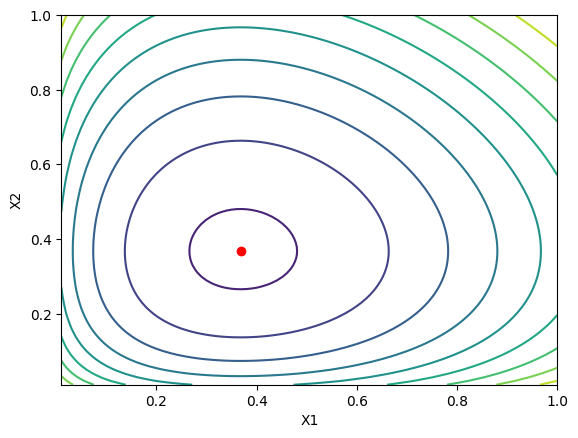
To check this, we can plot the function $G(X)$ for two variables $x_1$ and $x_2$ and see what it looks like.

The red dot is at the minimum at $x_1 = x_2 = 1/e$. Ok cool, so this was is a easy case to work with. Let’s use it to look at some other methods, that can be used here, but also in more general cases for either minimizing or solving a system of equations numerically. ..
Gradient Descent
The gradient descent or steepest descent method is a simple method we can use to find the minimum of a function or solve a system of equations (if we minimize the square of the residual in the system). The idea is to start at some guess and always take steps the direction that reduces the value of the objective function the most. There’s a million posts, blogs and papers on this, so I’m not going to belabor the point. We’re going to compute the gradient of the function and take steps in the direction of the negative gradient. For the function $G(X)$ above, we can compute the gradient as:
$$ \nabla G = \left[ \frac{\partial G}{\partial x_1}, \frac{\partial G}{\partial x_2} \right] = \left[ \ln(x_1) + 1, \ln(x_2) + 1 \right] $$ We can then take steps in the direction of the negative gradient. To avoid overshooting or taking too large of a step, we can multiply the gradient by a small number called the step size or learning rate. This is a ‘hyperparameter’ that you can tune to make the algorithm converge faster or slower. The update looks like this:
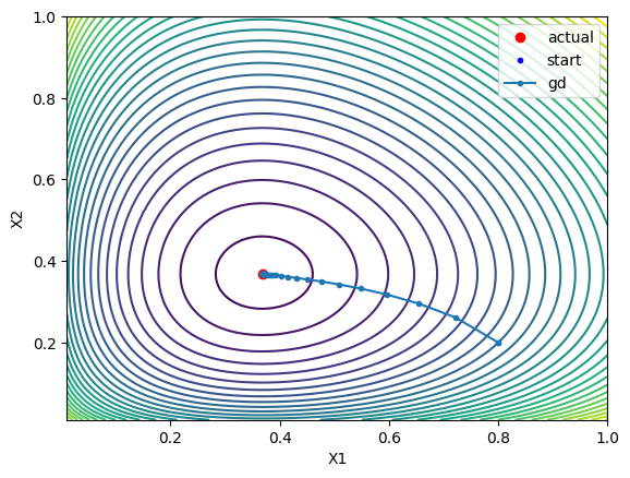
$$ X_{n+1} = X_n - \alpha \nabla G $$ where $\alpha$ is the learning rate. We can plot the steps that the algorithm takes to converge to the minimum:

Which is pretty cool! If you’re interested, this is what it looks like in code:
import numpy as np

def dg(x):
  return np.log(x) + 1.0

step_size = learning_rate = 0.1 # hyperparameter
x = np.array([0.8, 0.2]) # initial guess

# gradient descent
residual = 1.0
while residual > 1e-8:
  residual = np.dot(dg(x).T, dg(x))
  x = x - step_size * dg(x)
The good thing about this method is that it’s easy to implement and we’re always moving in the direction of ‘steepest descent’ - the direction that reduces the value of the function the most. The bad thing is that it can be slow to converge, especially if the function is ‘flat’ near the minimum. You can see in that there are a lot of steps taken near the minimum, which is inefficient.
This algorithm converges linearly, which means that the error decreases by a constant factor at each iteration. There’s another popular method called the Newton-Raphson method which converges quadratically, so that the error decreases much faster at each iteration.
Gradient descent finds a local minimum of the function we’re interested in. Newton-Raphson is a root finding method be can be used to find critical points, including minima, if we take the derivatives of the function we’re interested in and set them to zero, and apply Newton Raphson to the resulting system of equations.
Newton-Raphson
To use the Newton-Raphson method to minimize our test function $G(X)$, we need to write it as a system of equations. We can do this by taking the partial derivatives of $G$ with respect to each $x_i$ and setting them equal to zero, so that we have an equation for each $x_i$: $$ \frac{\partial G}{\partial x_i} = \ln(x_i) + 1 = 0 $$ Our new system, $F(X)$ is the system of equations above. For only two variables, we’ll have:
$$ F(X) = \begin{bmatrix} \ln(x_1) + 1 \\ \ln(x_2) + 1 \end{bmatrix} = 0 $$
An approximate ‘hand-wavy’ way to see how we can continue to think of a linear approximation to the function near the minimum, so something like a truncated Taylor series:
$$ F(X) \approx F(X_0) + DF(X_0) \cdot (X - X_0) $$
Where $DF(X_0)$ is the “Jacobian” of $F$ at $X_0$, or a matrix of where the rows correspond to the equations in $F$ and the columns correspond to the partial derivatives of each equation with respect to each variable. For example:
$$ DF = \begin{bmatrix} \frac{\partial F_1}{\partial x_1} & \dots & \frac{\partial F_1}{\partial x_n} \\ \vdots & \ddots & \ \vdots \\ \frac{\partial F_m}{\partial x_1} & \dots & \frac{\partial F_m}{\partial x_n} \\ \end{bmatrix} $$
or in our specific using our example with two variables, the Jacobian is:
$$ DF = \begin{bmatrix} \frac{1}{x_1} & 0 \\ 0 & \frac{1}{x_2} \end{bmatrix} $$
We can take that linear approximation and rearrange it to solve for $X$:
$$ X = X_0 - DF(X_0)^{-1} \cdot F(X_0) $$
Which gives the update rule that we need for Newton’s method. We can also write this a different way, as a linear system of equations, which is the way that it is usually implemented (to avoid inverting the Jacobian):
$$ DF(X_0) \cdot \Delta X = -F(X_0) $$
Which we can solve for $\Delta X$ and update $X$ as:
$$ X = X_0 + \Delta X $$
This is what it looks like in code:
def jacobi(x):
  j = np.zeros((x.shape[0], x.shape[0]))
  np.fill_diagonal(j, 1/x)
  return j

# newton raphson
x = np.array(x0)
residual = 1.0
while residual > 1e-8:
  residual = np.dot(dg(x).T, dg(x))
  dx = np.linalg.solve(jacobi(x), -dg(x))
  x = x + dx
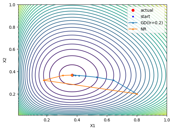
And with our test function, here’s the steps look like:

So it converges fast on it’s own and we don’t need to tune the learning rate as we did with gradient descent (it diverges or bounces around if the step size / learning rate is too high). However, we need to compute the Jacobian here, which is really the second derivatives of the original function we were working (it’s the Hessian wrt our test function $G(X)$), which can more difficult or less efficient to compute. Still, Newton’s method usually converges quadratically, or it does when it’s “sufficiently close” to the minimum and some other criteria are met.
These methods can be combined to get the benefits of each. For example: trying to use Newton’s method, but falling back to gradient descent if the the function at the new point is much different than what we expected.
There are a lot algorithms developed to improve the Newton-Raphson method, especially far from the solution (Trust region methods) and to avoid direct computation of the Hessian (the Jacobian in our example above) (Quasi-Newton Methods).
Of course they’re all implemented, in packages like scipy.optimize, Matlab,
etc, so you’ll never have to implement them yourself. But it’s interesting to
understand the basics about them.
So far, we’re only looking at unconstrained optimization, but there are a lot of cases where we have some constraints on the variables that we need to satisfy. For example, maybe in our test function $G(X)$, we need to find the minimum in the function where all $x_i$ need to add up to 1. How do we handle that?
Constrained Optimization
The methods that I’m familiar with for handling optimization problems with constraints basically involve transforming the problem into an unconstrained problem and then solving it the same way we did above. The Lagrange Multiplier method is one way to do this.
We can handle optimization subject to some equality constraints using the Lagrange Multiplier method. The idea is to take the function we want to optimize, in our case $G(X)$, and add each constraint, multiplied by a new variable, called the Lagrange Multiplier, $\lambda$. We then minimize this new function, which is called the Lagrangian, with respect to all the variables (the original variables $X$ and the Lagrange Multiplier(s) $\lambda$), instead of minimizing just the original function. So for example, we want to minimize:
$$ G(X) \quad \text{subject to} \quad \sum_i x_i = 1 $$
So we write the Lagrangian as:
$$ L(X, \lambda) = G(X) + \lambda \left( \sum_i x_i - 1 \right) $$ If we had more constraints, we would add them to the Lagrangian in the same way, each with a new Lagrange Multiplier. Then minimize the Lagrangian with respect to all the variables by taking the partial derivatives with respect to each one and setting them to zero. This gives us a system of equations to solve, which we can do using either of the methods we introduced above, or in some cases we can solve it analytically (like our toy problem above with $G(X)$). It does take a little extra work if we want to apply gradient descent, because the point that we’re looking is not a local minimum of the Lagrangian, but a saddle point. I don’t understand why it works, but you can apply gradient descent to the ‘x’ values, and gradient ascent to the Lagrange Multiplier(s) and it will become stable and converge to the minimum (example below, after introducing the Lagrangian for this specific example). This is presented in this paper.
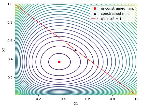
For two variables, we we want to minimize $G(X)$ subject to the constraint that $x_1 + x_2 = 1$, so we want to find the minimum of $G(X)$ along the red line in the plot below:

To apply the method of Lagrange Multipliers, we write the Lagrangian as:
$$ L(X, \lambda) = x_1\ln(x_1) + x_2\ln(x_2) + \lambda \left( x_1 + x_2 - 1 \right) $$ And then take the partial derivatives with respect to each variable and the Lagrange Multiplier and set them to zero. This gives us a system of equations: $$ \begin{align*} \frac{\partial L}{\partial x_1} &= \ln(x_1) + 1 + \lambda = 0 \\ \frac{\partial L}{\partial x_2} &= \ln(x_2) + 1 + \lambda = 0 \\ \frac{\partial L}{\partial \lambda} &= x_1 + x_2 - 1 = 0 \end{align*} $$ This case is pretty simple to work out analytically, if we wanted to get more practice, we could use the methods we introduced above to solve it numerically to make sure we get the same answer.
For this case:
$$ x_1 = e^{\lambda - 1}\\ x_2 = e^{\lambda - 1}\\ 2e^{\lambda - 1} = 1 \implies \lambda = \ln(1/2) + 1 \implies x_1 = x_2 = 1/2 $$
This new minimum is marked by the black triangle in the plot above.
We can actually show that in general, the solution for the minimum of $G(X)$ with any number of variables $n$ subject to the constraint that they all add up to 1 is $x_i = 1/n$ for all $i$
We can’t apply un modified gradient descent directly because the constrained minimum is not a local minimum of the Lagrangian, but a saddle point. If we wanted to use gradient descent we could run it on the square of the gradient of the Lagrangian instead of the Lagrangian itself, which would give us the minimum.
There is also a simpler the trick mentioned above and presented in this paper that we can apply here. It’s essentially the same thing we would do to apply gradient descent to the Lagrangian, but the Lagrange multiplier(s) are updated with gradient ascent instead of descent, eg we just add instead of subtract.
For this problem it looks like:
def dgc(x):
  d = np.zeros(x.shape)
  d[:2] = np.log(x[:2]) + 1 + x[2]
  d[2] = sum(x[:2]) - 1
  return d

# starting guess
x = np.array([0.8, 0.2, 0.0])
step_size = 0.2

# everything is descent, except last variable
dir = -1.0 * np.ones(x.shape)
dir[2] = 1.0

residual = 1.0
while residual > eps:
  residual = np.dot(dgc(x).T, dgc(x))
  x = x + dir * step_size * dgc(x)
print(x) # [0.5, 0.5, -0.3069]
Ok, so that’s a quick overview of the simplest versions in more than one variable of (1) two of the iterative methods that can be applied to optimization problems (gradient descent –> local min, Newton-Raphson –> find zeros, so it can be used to find critical points), and (2) how to formulate an optimization problem subject to constraints using the method of Lagrange Multipliers.
Here’s another example!
Example: Water-Gas Shift Reaction
The water-gas shift reaction is an important reaction in many industrial processes, including the production of hydrogen. It’s also convenient because it’s very simple and we can use it to test / illustrate the methods we’re talking about here.
Let’s say we want to compute the equilibrium concentrations of the species in the water-gas shift reaction, under some conditions and initial concentrations of water and carbon monoxide.
The reaction is: $$ CO + H_2O \rightleftharpoons CO_2 + H_2 $$
You’ll have to take my word for it because it’s a little out of scope for this post, but the reaction proceeds until the Gibbs free energy of the system is minimized. The Gibbs free energy in this system is given by (under some assumptions - gas phase reaction, ideal gas behavior):
$$ \frac{nG}{RT} = \sum_i n_i (\frac{G_i^*}{RT} + \ln(\frac{n_iP}{nP^0})) $$
where $n_i$ is the number of moles of species $i$, $G_i^*$ is the Gibbs free energy of formation of species $i$, (adjusted to temperature of interest - out of scope, a little tedious but straightforward), $P$ is the total pressure, and $P^0$ is the standard pressure (1 bar usually). So in terms of the actual minimization exercise, we only care about the mole numbers, the rest are constants.
Here, we do have a constraint, that the total number of moles of all elemental species is constant - eg we need to do a mass balance on each of the elements in the system. Then we can use the method of Lagrange Multipliers to write the Lagrangian: $$ L = \sum_i^{nc} n_i (\frac{G_i^*}{RT} + \ln(\frac{n_iP}{nP^0})) + \sum_i^{nc} \sum_j^{ne}\lambda_j (a_{ij}n_i - n_j^0) $$ Where the $\lambda_j$ are the Lagrange Multipliers for each element balance, and $a_{ij}$ is the stoichiometric coefficient of the element $j$ in species $i$.
If we differentiate the the Lagrangian with respect to each species mole number we end up with seven equations to solve, for the seven variables: the mole numbers of the species in the system, and the Lagrange Multiplier for each element balance constraint.
Our system of equations is:
$$ \begin{align*} \frac{\partial L}{\partial n_{i}} &= \frac{G_i^*}{RT} + \ln(\frac{n_iP}{nP^0}) + \sum_j^{ne}\lambda_j a_{ij} = 0 \quad \text{for} \quad i = 1, \dots, nc \\ \frac{\partial L}{\partial \lambda_{j}} &= \sum_i^{nc} a_{ij}n_i - n_j^0 = 0 \quad \text{for} \quad j = 1, \dots, ne \end{align*} $$
This is a system of nonlinear equations that we could solve using the methods
we introduced above. Those are little more involved in this case, so lets see
how we can lean on the packages like scipy.optimize to do the hard work for
us, given that we now have a rough idea of how they work, at least on a high
level.
The full code for this example is available as a gist, but this is the main part:
def lagrange(x):
  # Returns the system of equations we got by differentiating the
  # Lagranian and setting all the partial derivatives to zero
  # This uses 'lagrange mulipliers' to enforce the mass balance
  # constraints, but not to enforce the ni > 0 constraint, we could
  # use homotopy for that (maybe another post or continuation)
  #
  n = np.sum(x[:4]) # total moles
  # these are the partial derivatives of (nG/RT) wrt each species
  g = gf + np.log(x[:4]/n) + np.log(p) + np.matmul(x[4:], aij)
  # these are the constraints from element balance (the partial
  # derivatives wrt to the lagrange multipiers end up just
  # being the constaints)
  constraints = np.matmul(aij, x[:4]) - n_element_tot
  return np.concatenate((g, constraints))

def jac(x):
  # for scipy minimize if we want
  n = np.sum(x[:4])
  return gf + np.log(x[:4]/n) + np.log(p)

# this is a guess of the solution
# n is [nco, nco2, nh2o, nh2, lc, lh, lo]
n0 = np.array([1.0, 1.0, 1.0, 1.0, 1.0, 1.0, 1.0])

# Solve the lagrange problem lagrange((n, l)) = 0
#   this will tell us if we formulated correctly:
res = scipy.optimize.fsolve(lagrange, n0)
print("LM scipy fsolve: ", res[:4]/sum(res[:4]))
print("  ni:", res[:4])
print("  lambda:", res[4:])

# Turns out, we don't actually need to build the constraints into
# the function we pass to scipy.optimize, we can just pass them in
# as constraints and scipy will handle it for us. We can also pass
# in the jacobian if we want, if we don't, it will use numerical
# derivatives.
# Using built in minimization with constraints
cons = ({
  'type': 'eq',
  'fun': lambda x: np.matmul(aij, x) - n_element_tot
  },
)
res = scipy.optimize.minimize(
  gibbs, n0[:4], constraints=cons, jac=jac)
print(
  "\nMinimize (constained) our derivatives:",
  res.x/np.sum(res.x))
print(res)

res = scipy.optimize.minimize(
  gibbs, n0[:4], constraints=cons)
print(
  "\nMinimize (constained) numerical derivates:",
  res.x/np.sum(res.x))
print(res)
This is way overkill for this problem, we can also solve it analytically using the ‘reaction extent’ method, and we get the same answer. In general minimizing the Gibbs Free Energy is more flexible, and can be used to solve much more complex problems.
So that’s a quick overview of some common numerical methods that can be used for optimization problems involving functions of more than one variable, or for solving systems of nonlinear equations.